|
|
||
|---|---|---|
| doc | ||
| econml | ||
| monte_carlo_tests | ||
| notebooks | ||
| prototypes | ||
| .gitignore | ||
| LICENSE | ||
| README.md | ||
| azure-pipelines-steps.yml | ||
| azure-pipelines.yml | ||
| setup.cfg | ||
| setup.py | ||
README.md
 EconML: A Python Package for ML-Based Heterogeneous Treatment Effects Estimation
EconML is a Python package for estimating heterogeneous treatment effects from observational data via machine learning. This package was designed and built as part of the ALICE project at Microsoft Research with the goal to combine state-of-the-art machine learning techniques with econometrics to bring automation to complex causal inference problems. The promise of EconML:
- Implement recent techniques in the literature at the intersection of econometrics and machine learning
- Maintain flexibility in modeling the effect heterogeneity (via techniques such as random forests, boosting, lasso and neural nets), while preserving the causal interpretation of the learned model and often offering valid confidence intervals
- Use a unified API
- Build on standard Python packages for Machine Learning and Data Analysis
One of the biggest promises of machine learning is to automate decision making in a multitude of domains. At the core of many data-driven personalized decision scenarios is the estimation of heterogeneous treatment effects: what is the causal effect of an intervention on an outcome of interest for a sample with a particular set of features? In a nutshell, this toolkit is designed to measure the causal effect of some treatment variable(s) T on an outcome
variable Y, controlling for a set of features X. The methods implemented are applicable even with observational (non-experimental or historical) datasets.
For detailed information about the package, consult the documentation at https://econml.azurewebsites.net/.
For information on use cases and background material on causal inference and heterogeneous treatment effects see our webpage at https://www.microsoft.com/en-us/research/project/econml/
Table of Contents
News
November 18, 2020: Release v0.8.0, see release notes here
Previous releases
September 4, 2020: Release v0.8.0b1, see release notes here
March 6, 2020: Release v0.7.0, see release notes here
February 18, 2020: Release v0.7.0b1, see release notes here
January 10, 2020: Release v0.6.1, see release notes here
December 6, 2019: Release v0.6, see release notes here
November 21, 2019: Release v0.5, see release notes here.
June 3, 2019: Release v0.4, see release notes here.
May 3, 2019: Release v0.3, see release notes here.
April 10, 2019: Release v0.2, see release notes here.
March 6, 2019: Release v0.1, welcome to have a try and provide feedback.
Getting Started
Installation
Install the latest release from PyPI:
pip install econml
To install from source, see For Developers section below.
Usage Examples
Estimation Methods
Double Machine Learning (click to expand)
- Linear final stage
from econml.dml import LinearDML
from sklearn.linear_model import LassoCV
from econml.inference import BootstrapInference

est = LinearDML(model_y=LassoCV(), model_t=LassoCV())
### Estimate with OLS confidence intervals
est.fit(Y, T, X=X, W=W) # W -> high-dimensional confounders, X -> features
treatment_effects = est.effect(X_test)
lb, ub = est.effect_interval(X_test, alpha=0.05) # OLS confidence intervals

### Estimate with bootstrap confidence intervals
est.fit(Y, T, X=X, W=W, inference='bootstrap')  # with default bootstrap parameters
est.fit(Y, T, X=X, W=W, inference=BootstrapInference(n_bootstrap_samples=100))  # or customized
lb, ub = est.effect_interval(X_test, alpha=0.05) # Bootstrap confidence intervals
- Sparse linear final stage
from econml.dml import SparseLinearDML
from sklearn.linear_model import LassoCV

est = SparseLinearDML(model_y=LassoCV(), model_t=LassoCV())
est.fit(Y, T, X=X, W=W) # X -> high dimensional features
treatment_effects = est.effect(X_test)
lb, ub = est.effect_interval(X_test, alpha=0.05) # Confidence intervals via debiased lasso
- Nonparametric last stage
from econml.dml import ForestDML
from sklearn.ensemble import GradientBoostingRegressor

est = ForestDML(model_y=GradientBoostingRegressor(), model_t=GradientBoostingRegressor())
est.fit(Y, T, X=X, W=W)
treatment_effects = est.effect(X_test)
# Confidence intervals via Bootstrap-of-Little-Bags for forests
lb, ub = est.effect_interval(X_test, alpha=0.05)
Causal Forests (click to expand)
from econml.causal_forest import CausalForest
from sklearn.linear_model import LassoCV
# Use defaults
est = CausalForest()
# Or specify hyperparameters
est = CausalForest(n_trees=500, min_leaf_size=10,
                   max_depth=10, subsample_ratio=0.7,
                   lambda_reg=0.01,
                   discrete_treatment=False,
                   model_T=LassoCV(), model_Y=LassoCV())
est.fit(Y, T, X=X, W=W)
treatment_effects = est.effect(X_test)
# Confidence intervals via Bootstrap-of-Little-Bags for forests
lb, ub = est.effect_interval(X_test, alpha=0.05)
Orthogonal Random Forests (click to expand)
from econml.ortho_forest import DMLOrthoForest, DROrthoForest
from econml.sklearn_extensions.linear_model import WeightedLasso, WeightedLassoCV
# Use defaults
est = DMLOrthoForest()
est = DROrthoForest()
# Or specify hyperparameters
est = DMLOrthoForest(n_trees=500, min_leaf_size=10,
                     max_depth=10, subsample_ratio=0.7,
                     lambda_reg=0.01,
                     discrete_treatment=False,
                     model_T=WeightedLasso(alpha=0.01), model_Y=WeightedLasso(alpha=0.01),
                     model_T_final=WeightedLassoCV(cv=3), model_Y_final=WeightedLassoCV(cv=3))
est.fit(Y, T, X=X, W=W)
treatment_effects = est.effect(X_test)
# Confidence intervals via Bootstrap-of-Little-Bags for forests
lb, ub = est.effect_interval(X_test, alpha=0.05)
Meta-Learners (click to expand)
- XLearner
from econml.metalearners import XLearner
from sklearn.ensemble import GradientBoostingClassifier, GradientBoostingRegressor

est = XLearner(models=GradientBoostingRegressor(),
              propensity_model=GradientBoostingClassifier(),
              cate_models=GradientBoostingRegressor())
est.fit(Y, T, X=np.hstack([X, W]))
treatment_effects = est.effect(np.hstack([X_test, W_test]))

# Fit with bootstrap confidence interval construction enabled
est.fit(Y, T, X=np.hstack([X, W]), inference='bootstrap')
treatment_effects = est.effect(np.hstack([X_test, W_test]))
lb, ub = est.effect_interval(np.hstack([X_test, W_test]), alpha=0.05) # Bootstrap CIs
- SLearner
from econml.metalearners import SLearner
from sklearn.ensemble import GradientBoostingRegressor

est = SLearner(overall_model=GradientBoostingRegressor())
est.fit(Y, T, X=np.hstack([X, W]))
treatment_effects = est.effect(np.hstack([X_test, W_test]))
- TLearner
from econml.metalearners import TLearner
from sklearn.ensemble import GradientBoostingRegressor

est = TLearner(models=GradientBoostingRegressor())
est.fit(Y, T, X=np.hstack([X, W]))
treatment_effects = est.effect(np.hstack([X_test, W_test]))
Doubly Robust Learners (click to expand)
- Linear final stage
from econml.drlearner import LinearDRLearner
from sklearn.ensemble import GradientBoostingRegressor, GradientBoostingClassifier

est = LinearDRLearner(model_propensity=GradientBoostingClassifier(),
                      model_regression=GradientBoostingRegressor())
est.fit(Y, T, X=X, W=W)
treatment_effects = est.effect(X_test)
lb, ub = est.effect_interval(X_test, alpha=0.05)
- Sparse linear final stage
from econml.drlearner import SparseLinearDRLearner
from sklearn.ensemble import GradientBoostingRegressor, GradientBoostingClassifier

est = SparseLinearDRLearner(model_propensity=GradientBoostingClassifier(),
                            model_regression=GradientBoostingRegressor())
est.fit(Y, T, X=X, W=W)
treatment_effects = est.effect(X_test)
lb, ub = est.effect_interval(X_test, alpha=0.05)
- Nonparametric final stage
from econml.drlearner import ForestDRLearner
from sklearn.ensemble import GradientBoostingRegressor, GradientBoostingClassifier

est = ForestDRLearner(model_propensity=GradientBoostingClassifier(),
                      model_regression=GradientBoostingRegressor())
est.fit(Y, T, X=X, W=W)
treatment_effects = est.effect(X_test)
lb, ub = est.effect_interval(X_test, alpha=0.05)
Orthogonal Instrumental Variables (click to expand)
- Intent to Treat Doubly Robust Learner (discrete instrument, discrete treatment)
from econml.ortho_iv import LinearIntentToTreatDRIV
from sklearn.ensemble import GradientBoostingRegressor, GradientBoostingClassifier
from sklearn.linear_model import LinearRegression

est = LinearIntentToTreatDRIV(model_Y_X=GradientBoostingRegressor(),
                              model_T_XZ=GradientBoostingClassifier(),
                              flexible_model_effect=GradientBoostingRegressor())
est.fit(Y, T, Z=Z, X=X) # OLS inference by default
treatment_effects = est.effect(X_test)
lb, ub = est.effect_interval(X_test, alpha=0.05) # OLS confidence intervals
Deep Instrumental Variables (click to expand)
import keras
from econml.deepiv import DeepIVEstimator

treatment_model = keras.Sequential([keras.layers.Dense(128, activation='relu', input_shape=(2,)),
                                    keras.layers.Dropout(0.17),
                                    keras.layers.Dense(64, activation='relu'),
                                    keras.layers.Dropout(0.17),
                                    keras.layers.Dense(32, activation='relu'),
                                    keras.layers.Dropout(0.17)])
response_model = keras.Sequential([keras.layers.Dense(128, activation='relu', input_shape=(2,)),
                                  keras.layers.Dropout(0.17),
                                  keras.layers.Dense(64, activation='relu'),
                                  keras.layers.Dropout(0.17),
                                  keras.layers.Dense(32, activation='relu'),
                                  keras.layers.Dropout(0.17),
                                  keras.layers.Dense(1)])
est = DeepIVEstimator(n_components=10, # Number of gaussians in the mixture density networks)
                      m=lambda z, x: treatment_model(keras.layers.concatenate([z, x])), # Treatment model
                      h=lambda t, x: response_model(keras.layers.concatenate([t, x])), # Response model
                      n_samples=1 # Number of samples used to estimate the response
                      )
est.fit(Y, T, X=X, Z=Z) # Z -> instrumental variables
treatment_effects = est.effect(X_test)
See the References section for more details.
Interpretability
Tree Interpreter of the CATE model (click to expand)
from econml.cate_interpreter import SingleTreeCateInterpreter
intrp = SingleTreeCateInterpreter(include_model_uncertainty=True, max_depth=2, min_samples_leaf=10)
# We interpret the CATE model's behavior based on the features used for heterogeneity
intrp.interpret(est, X)
# Plot the tree
plt.figure(figsize=(25, 5))
intrp.plot(feature_names=['A', 'B', 'C', 'D'], fontsize=12)
plt.show()
Policy Interpreter of the CATE model (click to expand)
from econml.cate_interpreter import SingleTreePolicyInterpreter
# We find a tree-based treatment policy based on the CATE model
intrp = SingleTreePolicyInterpreter(risk_level=0.05, max_depth=2, min_samples_leaf=1,min_impurity_decrease=.001)
intrp.interpret(est, X, sample_treatment_costs=0.2)
# Plot the tree
plt.figure(figsize=(25, 5))
intrp.plot(feature_names=['A', 'B', 'C', 'D'], fontsize=12)
plt.show()
Inference
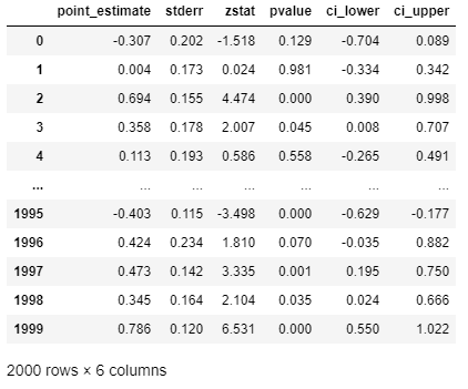
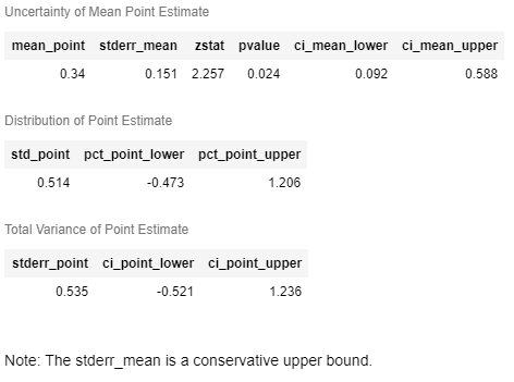
Whenever inference is enabled, then one can get a more structure InferenceResults object with more elaborate inference information, such
as p-values and z-statistics. When the CATE model is linear and parametric, then a summary() method is also enabled. For instance:
from econml.dml import LinearDML
# Use defaults
est = LinearDML()
est.fit(Y, T, X=X, W=W)
# Get the effect inference summary, which includes the standard error, z test score, p value, and confidence interval given each sample X[i]
est.effect_inference(X_test).summary_frame(alpha=0.05, value=0, decimals=3)
# Get the population summary for the entire sample X
est.effect_inference(X_test).population_summary(alpha=0.1, value=0, decimals=3, tol=0.001)
#  Get the inference summary for the final model
est.summary()
To see more complex examples, go to the notebooks section of the repository. For a more detailed description of the treatment effect estimation algorithms, see the EconML documentation.
For Developers
You can get started by cloning this repository. We use
setuptools for building and distributing our package.
We rely on some recent features of setuptools, so make sure to upgrade to a recent version with
pip install setuptools --upgrade. Then from your local copy of the repository you can run python setup.py develop to get started.
Running the tests
This project uses pytest for testing. To run tests locally after installing the package,
you can use python setup.py pytest.
Generating the documentation
This project's documentation is generated via Sphinx. Note that we use graphviz's
dot application to produce some of the images in our documentation, so you should make sure that dot is installed and in your path.
To generate a local copy of the documentation from a clone of this repository, just run python setup.py build_sphinx -W -E -a, which will build the documentation and place it under the build/sphinx/html path.
The reStructuredText files that make up the documentation are stored in the docs directory; module documentation is automatically generated by the Sphinx build process.
Blogs and Publications
-
June 2019: Treatment Effects with Instruments paper
-
May 2019: Open Data Science Conference Workshop
-
2017: DeepIV paper
Citation
If you use EconML in your research, please cite us as follows:
Microsoft Research. EconML: A Python Package for ML-Based Heterogeneous Treatment Effects Estimation. https://github.com/microsoft/EconML, 2019. Version 0.x.
BibTex:
@misc{econml,
  author={Microsoft Research},
  title={{EconML}: {A Python Package for ML-Based Heterogeneous Treatment Effects Estimation}},
  howpublished={https://github.com/microsoft/EconML},
  note={Version 0.x},
  year={2019}
}
Contributing and Feedback
This project welcomes contributions and suggestions. Most contributions require you to agree to a Contributor License Agreement (CLA) declaring that you have the right to, and actually do, grant us the rights to use your contribution. For details, visit https://cla.microsoft.com.
When you submit a pull request, a CLA-bot will automatically determine whether you need to provide a CLA and decorate the PR appropriately (e.g., label, comment). Simply follow the instructions provided by the bot. You will only need to do this once across all repos using our CLA.
This project has adopted the Microsoft Open Source Code of Conduct. For more information see the Code of Conduct FAQ or contact opencode@microsoft.com with any additional questions or comments.
References
V. Syrgkanis, V. Lei, M. Oprescu, M. Hei, K. Battocchi, G. Lewis. Machine Learning Estimation of Heterogeneous Treatment Effects with Instruments. Proceedings of the 33rd Conference on Neural Information Processing Systems (NeurIPS), 2019 (Spotlight Presentation)
D. Foster, V. Syrgkanis. Orthogonal Statistical Learning. Proceedings of the 32nd Annual Conference on Learning Theory (COLT), 2019 (Best Paper Award)
M. Oprescu, V. Syrgkanis and Z. S. Wu. Orthogonal Random Forest for Causal Inference. Proceedings of the 36th International Conference on Machine Learning (ICML), 2019.
S. Künzel, J. Sekhon, J. Bickel and B. Yu. Metalearners for estimating heterogeneous treatment effects using machine learning. Proceedings of the national academy of sciences, 116(10), 4156-4165, 2019.
V. Chernozhukov, D. Nekipelov, V. Semenova, V. Syrgkanis. Plug-in Regularized Estimation of High-Dimensional Parameters in Nonlinear Semiparametric Models. Arxiv preprint arxiv:1806.04823, 2018.
Jason Hartford, Greg Lewis, Kevin Leyton-Brown, and Matt Taddy. Deep IV: A flexible approach for counterfactual prediction. Proceedings of the 34th International Conference on Machine Learning, ICML'17, 2017.
V. Chernozhukov, D. Chetverikov, M. Demirer, E. Duflo, C. Hansen, and a. W. Newey. Double Machine Learning for Treatment and Causal Parameters. ArXiv preprint arXiv:1608.00060, 2016.


