customer-insights-azure-data-workshop/lab04.md

Lab 4 - Predicting Customer Churn in Azure Machine Learning

Contents

Introduction

Objectives

Step 1: Sign into Azure ML Studio and choose your workspace

Step 2: Create Data Connection and Dataset

Step 3: Experiment Design

Step 4: Training models

Step 5: Output Model

Lab Overview

Introduction

The purpose of this lab is to allow you to get hands-on experience creating an Azure Machine Learning model to predict which telecommunications customers are likely to churn (i.e. to stop using the service or move to a competitor). The output of this model will allow a targeted intervention to try to retain these customers since retaining existing customers is more cost effective than gaining new customers.

Objectives

The objectives of this exercise are to:

• Sign into Azure ML

• Create a datastore connected to Azure Synapse Serverless SQL

• Create a dataset from the datastore

• Learn how to prepare the data for machine learning

• Learn how to perform classification to predict whether a subscriber will churn.

• Learn how to train and evaluate a model

• Learn how to compare the accuracy of several models.

• Export the results of the models to Blob Storage

Estimated time for this lab is 75 minutes

Exercise 1: Creating a Telco Churn Model

This exercise uses an anonymized telecommunications dataset about customers to predict which customers will cancel their subscription. In the telecommunications industry, a subscriber cancelling is called “churn.”

Step 1: Sign into Azure ML Studio and choose your workspace

In this step, you will sign into Azure ML Studio and choose which workspace you will use for creating experiments.

1. Navigate to ml.azure.com in your browser. If you’re already signed in, you will be directed to the main Azure ML screen. If not, you will be asked to sign in.

   

2. Select your “amlworkspace<suffix>” Azure ML workspace you created in Lab 2 from the drop-down menu. Click the “Get started” button. You will be directed to the Azure ML home screen.

   

3. In the top right, there is a directory and workspace selection. Ensure you are in the desired directory, subscription and workspace.

   

Step 2: Create Data Connection and Dataset

In this step, you connect to Azure Synapse Serverless SQL using the Azure SQL database datastore type and perform a query to extract the data.

1. To connect to the data. Click the Datastores option on the left pane.

   

2. Choose + New Datastore

   

3. Enter the details of the new datastore. Name the Datastore “telcochurn” and select “Azure SQL Database” as the Datastore type. The server name will be “asaworkspace<suffix>-ondemand”. The Database name is “CI”. Select the proper Subscription ID and Resource Group assigned to your project “customer-insights-workshop-rg”. The User ID will be “asa.sql.admin”. Enter the password you created in lab 2. Select “No” on using the workspace managed identity for data preview. Once done, click “Create” at the bottom. Note: Even though the documented connection string for Synapse Serverless SQL is asaworkspace<suffix>-ondemand.sql.azuresynapse.net, asaworkspace<suffix>-ondemand.database.windows.net also works.

   

4. Upon creation, “telcochurn” will appear in the datastore selection, click on it to create a new dataset.

   

5. Select Create Dataset from the Overview screen

   

6. Give the dataset the name TelcoChurn and select Dataset Type as Tabular. Click Next.

   

7. Enter the following SQL Query into the space provided: select * from dbo.CustomerChurn. Leave Skip Data Validation UNCHECKED then click Next. This will connect to the data and pop up with a data preview screen. After the preview has loaded, click Next. Note: we could’ve also created the Datastore on this screen.

   

8. The next options are to set the Schema. Here we can set the data types of each column. Azure ML will automatically detect what it perceives the data type to be. We can accept the defaults and click Next.

   

9. The final step for creating the dataset is to Confirm the details. Review the screen and click Create at the bottom of the page.

   

10. Once complete, there will be a success notification.

    

Step 3: Experiment Design

In this step, you will add a dataset from the datastore and begin designing the experiment.

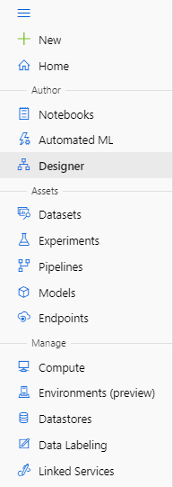
1. In the selection pane on the left, select the Designer module.

   

2. Select the New Pipeline option Easy-to-use-prebuilt modules

   

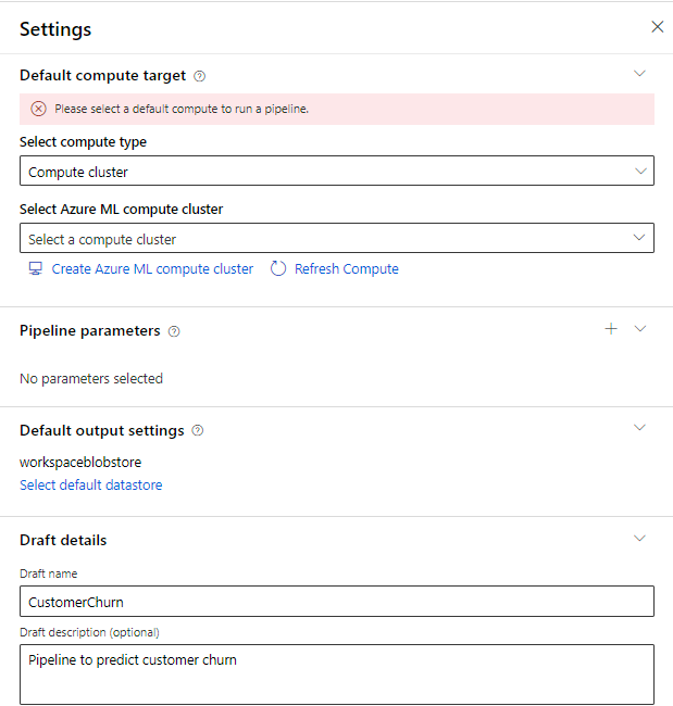
3. In the Settings pane that pops up on the right, we need to specify a compute cluster as well as pipeline settings. If you already have a compute cluster initiated, please skip down to step 8. Note: if the settings pane does not pop up automatically, select the gear icon next to the Pipeline name.

   

4. Select Compute Cluster for the compute type and then click Create Azure ML Compute Cluster.

   

5. In the Compute Cluster screen, we are going to select the default options of Dedicated Priority, CPU Virtual Machine, and Standard_DS3_v2. If Standard_DS3_v2 is not an option, click the ‘Select from all options’ and locate it then. The Location should be defaulted to your region but you can change that if necessary. Click Next when complete.

   

6. In the Advanced Settings, you will see your selections from the prior screen at the top. Name the compute CustomerChurnCC. Set the Minimum number of nodes at 0 and Maximum at 2. Set the Idle seconds before scale down to 60. Click Create when complete and wait a few minutes.

   

7. After creation, you will be redirected back to the Setting pane of the pipeline, select the newly created Compute Cluster from the options. If you have trouble selecting the compute cluster from the dropdown, wait until you receive a message saying “Compute ‘CustomerChurnCC’ provisioning succeeded” then try to select it again. Name the draft “CustomerChurn”

   

8. We are going to begin the process of dragging what are called assets or modules on the page to build a pipeline starting with data ingestion and ending in exporting the model results to the datastore.

   There are multiple ways to accomplish this task, we are going to build a basic pipeline for demonstration. In a real-world scenario, we would train multiple models and perform hyperparameter tuning to find the optimal model.

9. Let’s begin with bringing in the data set we created earlier. Open the Datasets module and drag the TelcoChurn dataset onto the designer page.

   

10. If you select the TelcoChurn asset on the designer page, you can see the details of it. Every asset will work similarly when selected. The only difference will be that some will require parameters to be set (We will cover this shortly).

    

11. Next, we know that TotalCharges has a few blank values (we could have tested this via using the Summarize Data asset and evaluating each column distribution but for the sake of this lab we’re going to move on to handling them). Search for Clean Missing Data:

    

    Drag Clean Missing Data onto the page and connect TelcoChurn to the new asset.

    

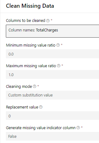
12. In the properties pane for Clean Missing Data. Click "Edit column" and select TotalCharges as the Column and set the parameters below. Note: If the goal of the lab was to build the best model we would have run some form of regression or sub-sample from the complete rows to find a predicted value for this.

    

13. Next, drag Split Data onto the page. Connect the left node of Clean Missing data to the top of Split Data as shown below. Set the parameters to match the following settings. To train a machine learning model, we need to provide data for the model to train on. Generally, we provide 25% of the data to train the model and then test on the remaining 75%. This ensures that we have a large enough dataset to test our proposed model on. You can set the Random seed to any number you’d like, or leave it blank. The seed is used for re-producibility of results.

    

14. From the Split Data asset, we are going to connect the left node (training) to 1 new asset and the right node (testing) to 3 new assets. The left node is connected to Select Columns in Dataset (drag over from the module options). Click "Edit column" to launch the Select columns dialog. In the Select columns options click the "By name" radio button and click "Add all":

    

    Remove the customerID column by clicking the minus sign next to it. If we were to leave the ID in, the models would treat that as a feature which would cause errors down the line.

    

    Your screen should look like this. Click Save.

    

    The selected columns should then be listed here:

    

15. The right node of the Split Data asset is connected to another instance of Select Columns in Dataset. This extracts the Customer ID’s of the testing data. We are going to join this back in to the results dataset after the models have run. Note that the description "Extract customer ID to join back in later" can be added in the Comment section of the properties pane of that module. This is optional.

    

16. We’re going to create two models. The first one is a Two-Class Boosted Decision Tree with the following parameters. Search for and drag Two-Class Boosted Decision Tree from the module selection over to the page. Yours will not turn green until after we have successfully run the pipeline

    

17. The second is a Two-Class Decision Forest with the following parameters. Drag this on to the page.

    

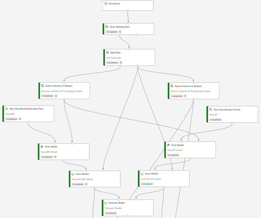
18. Checkpoint. Below is how our designer page looks for reference. Yours will not show the green Completed indicator on the models just yet. Those appear after we’ve ran the pipeline.

    

Step 4: Training models

Note: If you get confused on how modules should be connected, feel free to skip down to a zoomed-out screenshot in Step 5.7 below.

Now that we’ve setup the design of our experiment, we can begin to train the models and evaluate the outputs.

1. You will first train a Two-Class Boosted Decision Tree. Setup your page similarly to the one below. You should already have Split Data, Select Columns and the Decision Tree setup. Add a Train Model and Score Model step. Connect the Two-Class Boosted Decision Tree to the left node on Train Model and then the Select Columns in Dataset to the right node on Train Model. Connect the single output node of Train Model to the left node on Score Model and then the right output node of Split Data to the right input node on Score Model.

   

2. In the properties pane of the Train Model module, choose the Churn column since that is the column we are trying to predict.

   

3. Now add a Two-Class Decision Forest, along with another Train Model and Score Model. Connect the Two-Class Decision Forest output node to the left input node on Train Model and then the Select Columns in Dataset output node to the right input node on the Train Model. Finally add an Evaluate Model to the bottom and connect both Score Models to it.

   

4. Review the screenshot below to make sure all of the connections are made. Your page should look similar to this. Press the Submit button at the top right of the screen.

   

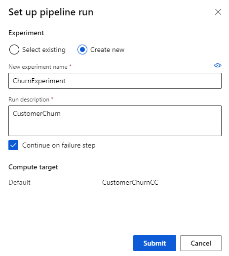
5. On the Set up pipeline run popup, create a new experiment and name it. Clicking Submit will kick off the run so we can evaluate the two models.

   

6. The pipeline run will take about 10-15 minutes on the sample data. Once complete, click on the Evaluate Model step and then the Output + Logs option. Then click the Evaluation results option.

   

7. From here, we can see the results of both models side by side to compare them. The Decision Tree was the left port and the Decision Forest was the right port. Without getting too thick into the weeds, we can see that the left port had a higher accuracy, precision, and AUC at the 0.5 threshold. Sliding the threshold back and forth changes the values. The right port received higher marks for Recall and F1 Score.

   

8. Naturally, we could go back to the parameters and introduce parameter sweeps, hyper-tuning, and feature selection to try and boost these scores. For the purposes of this lab, we are going to proceed with the baseline models.

Step 5: Output Model

In this step, we’re going to output the results of these models to blob storage for the next labs.

1. CHECK. Your page should look similar to this at this point in the lab.

   

2. Drag the following modules below the evaluate model step. Connect the Score Model for the Decision Tree to the left column and then the Score Model for the Decision Forest to the right column.

   

3. In the parameters for both Select Columns in Dataset, set the following. We only want to keep the Predicted Labels and Probabilities.

   

4. At the Add Columns step, we’re going to add back in the Customer ID’s that we extracted earlier from the testing dataset.

   

5. At the Convert to CSV stage, we are going to send the model results to Blob Storage as CSV’s. On the left side, change the output settings to the following with the Path on datastore as: azureml/Decision_Tree_Results/dtresults

   

6. On the right side set the Path to datastore as: azureml/Decision_Forest_Results/dfresults

7. The final designer should resemble this:

   

8. Once complete, hit Submit in the top right to begin the pipeline run. This should take approximately 3 to 5 minutes.

9. After completion, select one of the Convert to CSV modules and then Access Data

   

10. From here, you can see the data outputs. data.csv is the output file we’ll need in the next section. The URL for the file can be accessed by clicking on the file.

    

11. If you would like to view the data, you can select the Edit button to preview it.

12. Refer back to the Clean Missing Data module. In the Output Settings Option, we are going to select Regenerate Output. This will ensure that every time we execute the pipeline, we are re-executing the SQL query to pull the latest data and handling the missing values appropriately and not using cached results from a previous execution.

    

13. The final step is to Publish the pipeline. Click the Publish button in the top right next to the Submit button. Select Create New and call it CustomerChurnEP. Click Publish.

    

14. Click on the Pipelines tab to see the newly published pipeline.

    

    After approximately 60 seconds, the cluster will scale down (to ensure you do not incur any unnecessary costs) until another experiment is kicked off.

Summary

In this lab, you signed into Azure Machine Learning Studio, created a datastore connected to a SQL database, prepared the data, trained two models, evaluated the accuracy of the models, and sent the output of those models to Blob Storage to be accessed by other Microsoft resources. Classification tasks can easily be performed with Azure ML using Two-Class Boosted Decision Trees or Two-Class Decision Forests.

Next, go to Lab 5.